动手学AI ⚡️ 手写Transformer 01：环境与前期准备¶

系列目录¶

1. 环境准备¶

因为很多小白会卡在开头，这部分就冗余了一些。了解这些概念的同学直接跳到 Part 2。

1.1 Colab¶

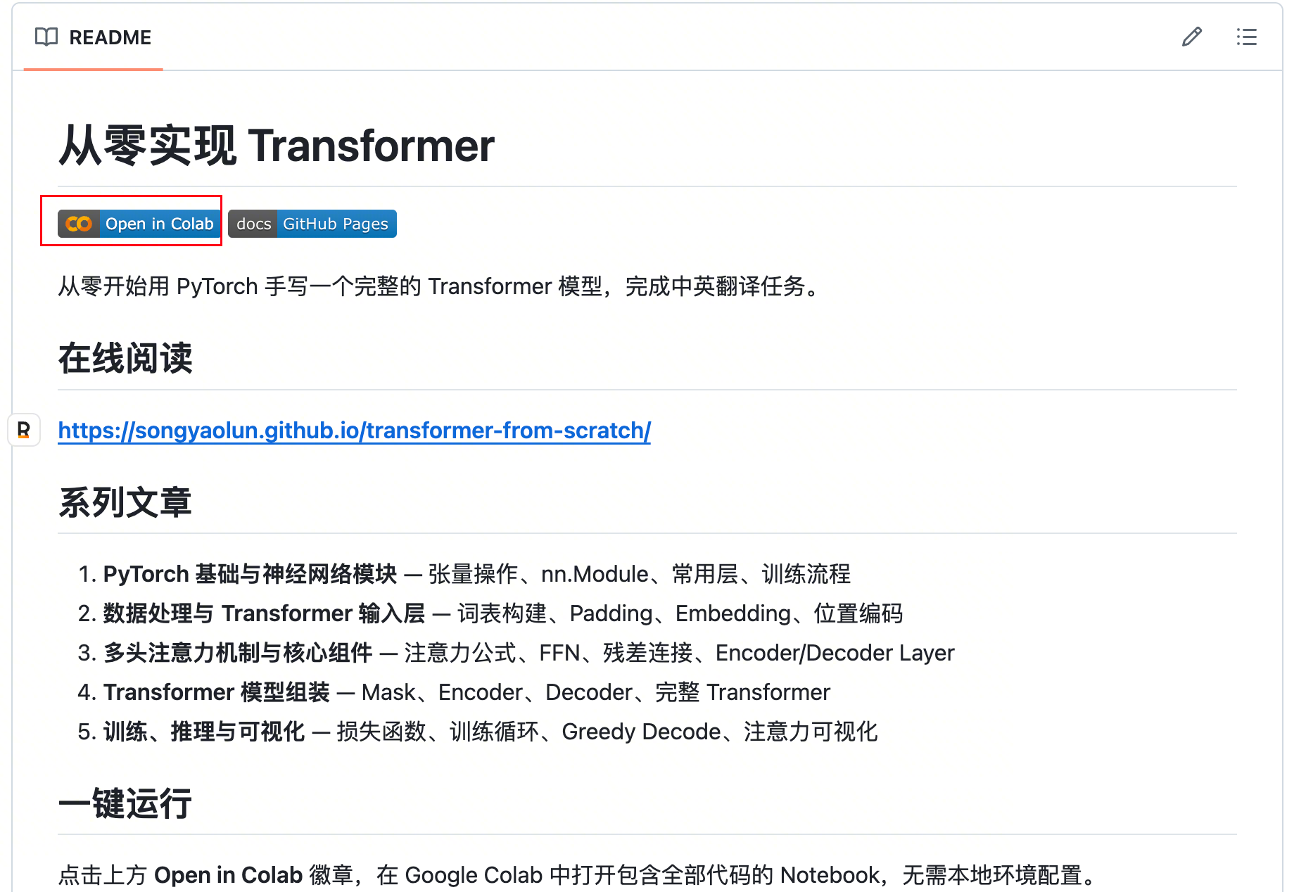
打开本系列关联的 Github 仓库：https://github.com/songyaolun/transformer-from-scratch，按以下步骤操作：

第一步，点击仓库中的 notebook 链接，在 Colab 中打开：

Colab 打开步骤1

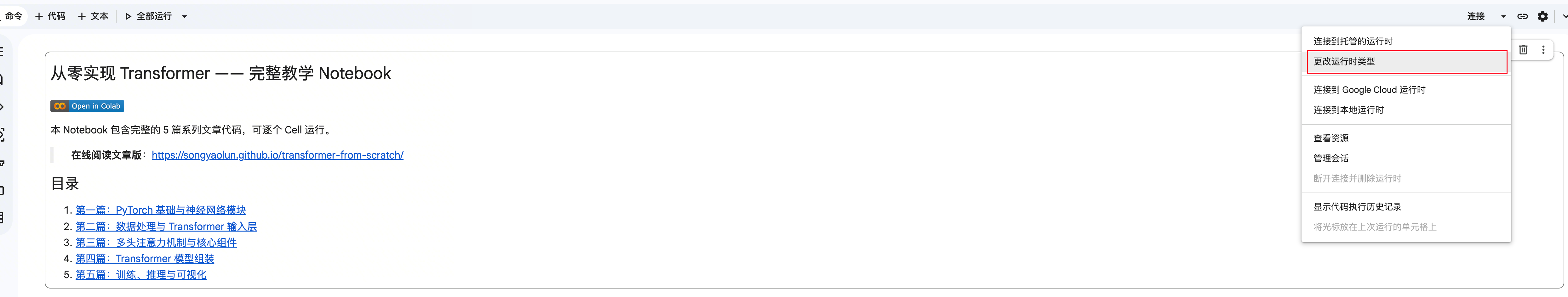
第二步，在跳转的新页面中选择右上角的小三角，选择更改运行时类型：

Colab 更改运行时

第三步，选择 T4 GPU 并保存：

选择 T4 GPU

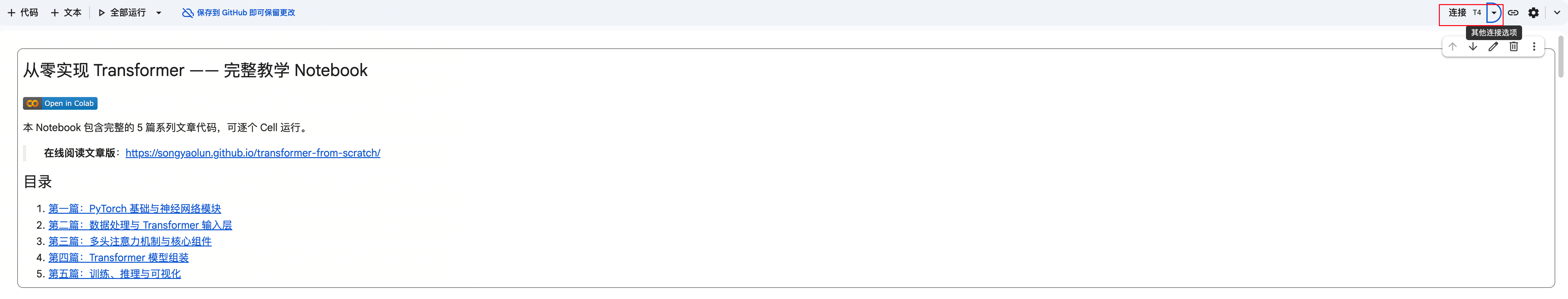
第四步，点击连接 T4，稍等几秒：

连接 T4

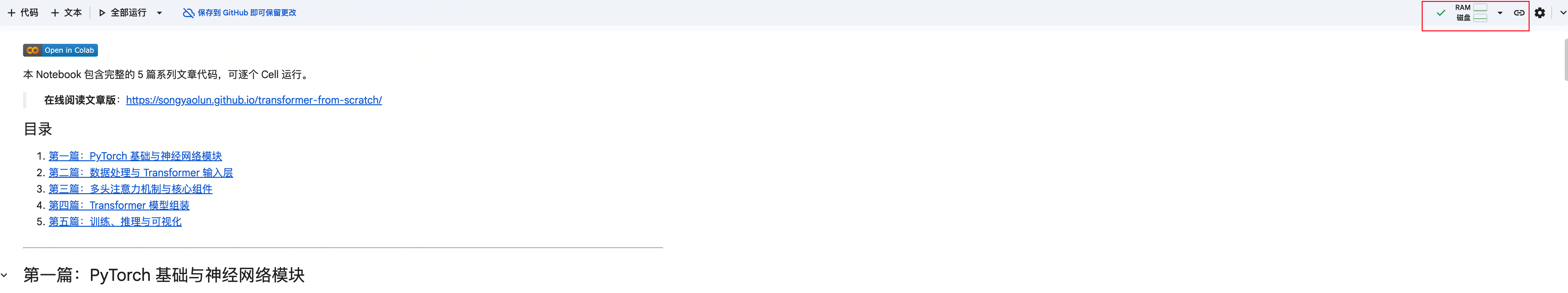
右上角出现 RAM 和磁盘，说明 Colab 已经连上了——给你分配了一台云端机器，有内存、有 GPU、有磁盘：

RAM 和磁盘显示

第五步，将下图的内容取消注释并运行，即可安装后文所需的全部依赖：

安装依赖

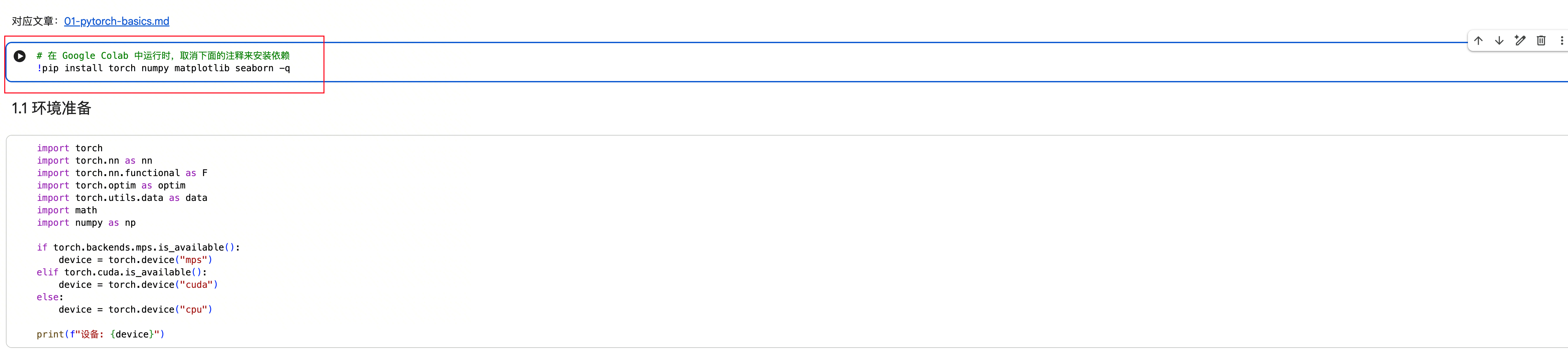
点击按钮开始运行代码：

运行代码

1.2 PyCharm / VS Code¶

需要先在本地配置环境，推荐使用 Conda，安装好依赖后，第一次运行 Cell 时会询问你环境配置，指定到具体的配置就好。以 VS Code 举例：

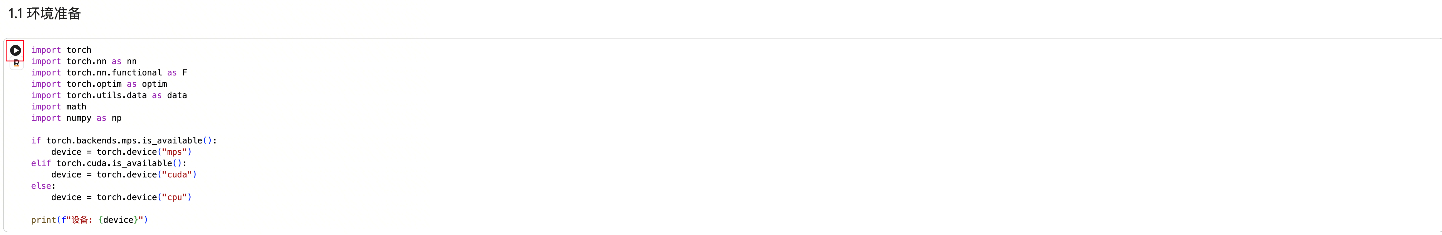
点击 cell 左侧的 Run 按钮：

VS Code 运行 Cell

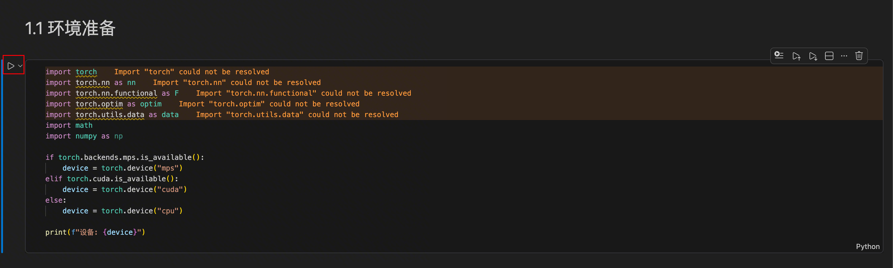
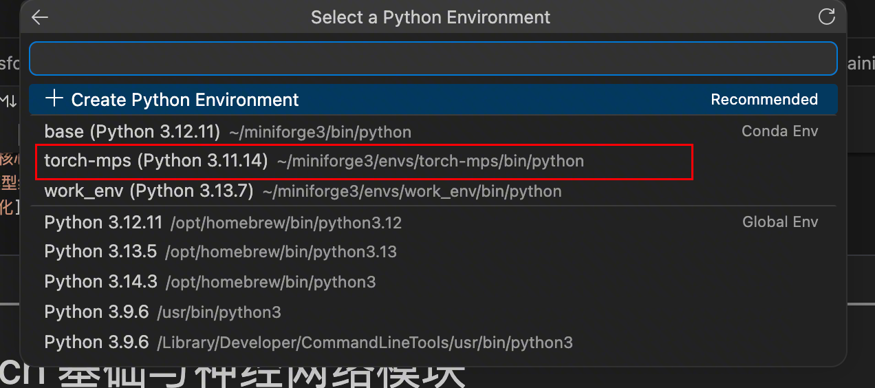
弹出环境配置选项：

选择环境

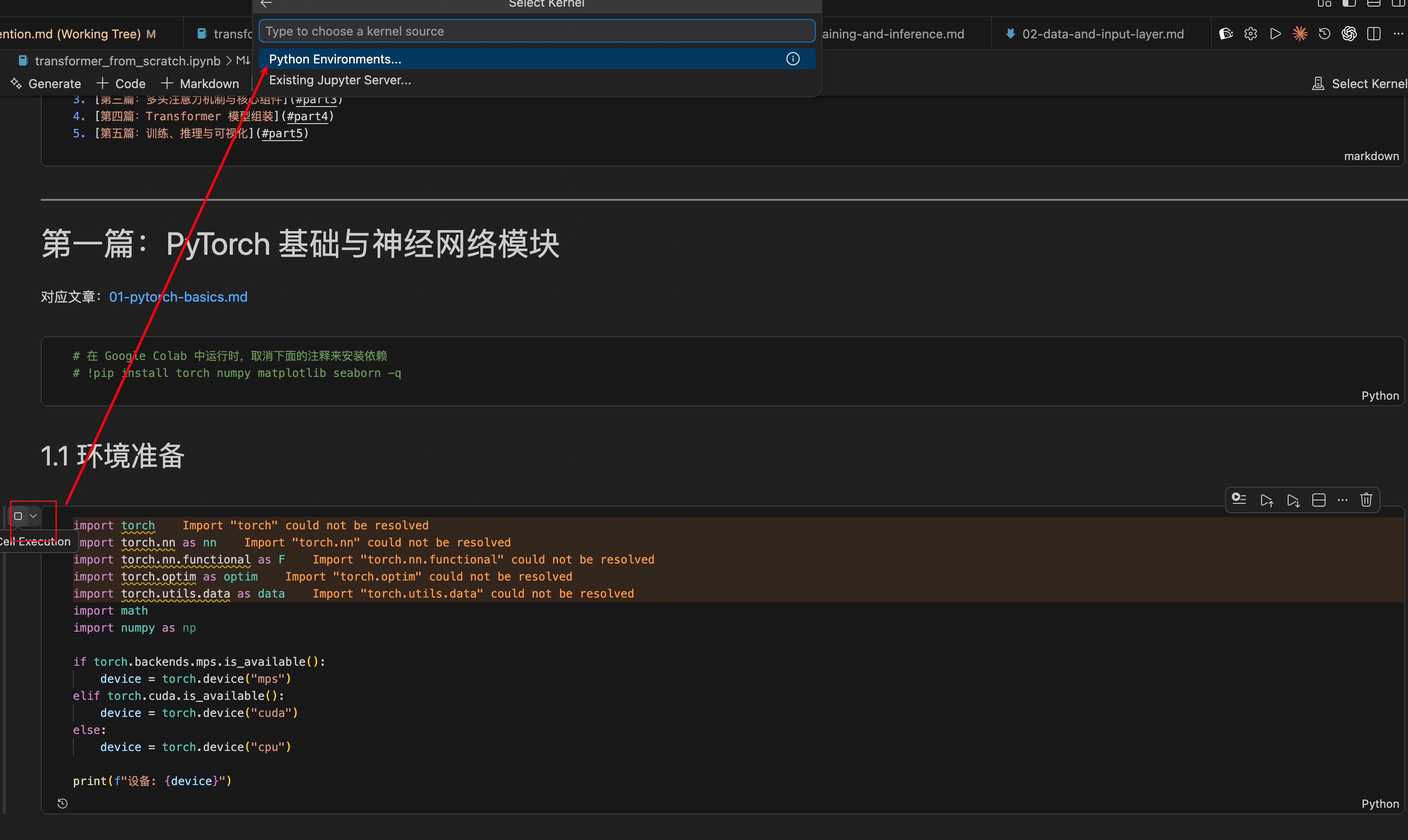
选择具体的环境（我用 Conda 专门建了一个）：

选择 Conda 环境

然后运行第一段代码：

import torch
import torch.nn as nn
import math

if torch.backends.mps.is_available():
    device = torch.device("mps")
elif torch.cuda.is_available():
    device = torch.device("cuda")
else:
    device = torch.device("cpu")

print(f"设备: {device}")

我的个人电脑是 M1 系列的 Mac，执行结果是 设备: mps。如果你用有 NVIDIA GPU 的电脑，或者使用 Colab 并选择了 Google 的免费 GPU，结果应该是 设备: cuda。

环境跑通了？下面正式开始。Transformer 的一切计算都建立在张量（Tensor）之上——你可以把它理解为多维数组的升级版。

2. 张量——AI 的积木¶

PyTorch 是当前深度学习的主流框架，类似于 Web 开发中的 React 或 Spring——帮你省掉重复劳动，专注核心逻辑。

创建张量¶

import torch

# 从列表创建
x = torch.tensor([1, 2, 3])
print(x)         # tensor([1, 2, 3])
print(x.shape)   # torch.Size([3])

# 从二维列表创建
matrix = torch.tensor([[1, 2], [3, 4]])
print(matrix)        # tensor([[1, 2], [3, 4]])
print(matrix.shape)  # torch.Size([2, 2])

常用的创建方法：

x = torch.zeros(2, 3)    # 全 0 张量
x = torch.ones(3, 2)     # 全 1 张量
x = torch.randn(3, 4)    # 标准正态分布张量

张量属性¶

x = torch.randn(2, 4, 5)
print(x.shape)    # torch.Size([2, 4, 5])
print(x.dim())    # 3 (维度)
print(x.numel())  # 40 (元素总数)
print(x.dtype)    # torch.float32 (数据类型)

张量索引¶

x = torch.tensor([[1, 2, 3], [4, 5, 6]])
print(x[0, 1])     # 2 (访问单个元素)
print(x[0])         # tensor([1, 2, 3]) (第一行)
print(x[:, 1:])     # tensor([[2, 3], [5, 6]]) (切片)

形状操作¶

view() — 变换形状¶

x = torch.randn(2, 3, 4)
x_flat = x.view(2, -1)         # (2, 12)，-1 自动推断
x_high = x_flat.view(2, 2, -1, 2)  # (2, 2, 3, 2)

什么时候用？拆分多头注意力的时候（不理解没关系，后面会讲）：

B, T, C = 2, 3, 8
x = torch.randn(B, T, C)
n_heads = 2
head_dim = C // n_heads
x_heads = x.view(B, T, n_heads, head_dim)  # (2, 3, 2, 4)

transpose() — 交换两个维度¶

x = torch.randn(2, 3, 4)
x_t = x.transpose(1, 2)  # (2, 4, 3)

permute() — 重排所有维度¶

x = torch.randn(2, 3, 4, 5)
x_p = x.permute(0, 3, 1, 2)  # (2, 5, 3, 4)

📖 transpose 和 permute 感觉差不多，为啥设计两个类似的方法呢？

transpose 源自矩阵转置，只交换两个维度，不感知其他维度；permute 可以一次重排所有维度。只需交换两个维度时，transpose(0, 1) 写法简洁，不必像 permute(1, 0, 2, 3, 4, ...) 那样罗列全部维度——维度越多差距越明显。反过来，需要重排多个维度时，permute 一行搞定，transpose 则要链式调用多次。

真实 Transformer 中的用法：

B, T, C = 2, 3, 512
n_head = 8
head_dim = C // n_head
x = torch.randn(B, T, C)
x = x.view(B, T, n_head, head_dim)
x = x.permute(0, 2, 1, 3)  # (2, 8, 3, 64)

unsqueeze() / squeeze() — 增/减维度¶

函数名本身就很直观——squeeze 有"挤压"的意思。squeeze() 去掉所有大小为 1 的维度，就像把空气从包装袋里挤出去；unsqueeze() 则是在指定位置插入一个大小为 1 的维度。

x = torch.tensor([1, 2, 3])   # shape: (3,)
x1 = x.unsqueeze(0)           # shape: (1, 3)，在第0维增加
x2 = x.unsqueeze(1)           # shape: (3, 1)，在第1维增加

x = torch.randn(1, 3, 1, 4)  # shape: (1, 3, 1, 4)
x = x.squeeze()                # shape: (3, 4)，删除所有大小为 1 的维度

📖 为什么有了 view 还要 squeeze/unsqueeze？

因为 unsqueeze(1) 不需要关心其他维度的 size，而 view 必须声明所有维度的值。

torch.cat() — 拼接张量¶

x1 = torch.tensor([[1, 2, 3], [4, 5, 6]])
x2 = torch.tensor([[7, 8, 9], [10, 11, 12]])

torch.cat([x1, x2], dim=0)  # (4, 3)
torch.cat([x2, x1], dim=1)  # (2, 6)

contiguous() — 确保内存连续¶

x = torch.randn(2, 3, 4)
x = x.transpose(0, 1)  # 转置后内存不连续
# x.view(2, 4, 3)  # 报错！
x = x.contiguous()
x = x.view(2, 4, 3)    # 正常

transpose、permute 等操作改变的是内存布局，而 view 要求内存连续，所以需要 contiguous()——就像书的页码乱了，view 要求页码连续才能重新装订。

矩阵运算¶

a = torch.tensor([[1, 2, 3], [4, 5, 6]])
b = torch.tensor([[7, 8], [9, 10], [11, 12]])

a @ b              # 等价于 torch.matmul(a, b)
# tensor([[ 58,  64],
#         [139, 154]])

# 批量矩阵乘法
A = torch.randn(10, 2, 3)
B = torch.randn(10, 3, 4)
C = torch.matmul(A, B)  # (10, 2, 4)

掩码操作¶

x = torch.randn(2, 3)
mask = torch.tensor([[True, False, True], [False, True, False]])
result = x.masked_fill(mask, -1e9)  # mask 为 True 的位置填 -1e9

三角掩码（Transformer 中用于防止看到未来信息）：

x = torch.ones(4, 4)
torch.triu(x)  # 上三角
torch.tril(x)  # 下三角

比较操作¶

# eq() 等于 | ne() 不等于 | gt() 大于 | ge() 大于等于 | lt() 小于 | le() 小于等于

x = torch.tensor([1, 0, 3, 0, 5])
mask = x.ne(0)  # 不等于 0 的位置为 True
print(f"不等于0的位置: {mask}")

3. nn.Module——搭积木的方式¶

nn.Module 是所有神经网络的基类，类似于 Java 的 Object 类。

3.1 基本结构¶

import torch.nn as nn

class MyModel(nn.Module):
    def __init__(self):
        super().__init__()           # 必须调用！
        self.linear = nn.Linear(10, 5)

    def forward(self, x):
        return self.linear(x)

model = MyModel()

super().__init__() 是必须调用的，它初始化了参数注册、buffer 管理等功能。如果不调用，会直接报错：

class BrokenModel(nn.Module):
    def __init__(self):
        self.linear = nn.Linear(10, 5)  # AttributeError!

3.2 完整的调用链演示¶

class MyLayer(nn.Module):
    def __init__(self, in_features, out_features, name="MyLayer"):
        super().__init__()
        self.weight = nn.Parameter(torch.randn(out_features, in_features))
        self.name = name
        print(f"MyLayer 初始化完成，weight shape: {self.weight.shape}")

    def forward(self, x):
        print(f"MyLayer {self.name} 的forward被调用，input shape: {x.shape}")
        return x @ self.weight.t()


class MyModel(nn.Module):
    def __init__(self, in_features, out_features):
        super().__init__()
        self.layer1 = MyLayer(in_features, 40, "layer1")
        self.layer2 = MyLayer(40, 5, "layer2")

    def forward(self, x):
        print(f"MyModel 的forward被调用，input shape: {x.shape}")
        x = self.layer1(x)
        x = torch.relu(x)
        return self.layer2(x)


model = MyModel(10, 20)
x = torch.randn(2, 10)
output = model(x)

调用链路：

model(x) → model.__call__(x) → model.forward(x) → self.layer1(x)
  → layer1.__call__(x) → layer1.forward(x) → relu(x) → self.layer2(x)
  → layer2.__call__(x) → layer2.forward(x)

📖 为什么调用 model(x)，不直接调用 model.forward(x) 呢？

当你运行 model(x) 时，Python 实际调用的是 model.__call__(x)。在 nn.Module 的 __call__ 方法中，会先运行各种 Hook，最后才调用你写的 forward(x)。

# nn.Module 的简化实现（仅供理解）
class Module:
    def __call__(self, *args, **kwargs):
        # 1. 执行前置操作（各种 Hook）
        result = self.forward(*args, **kwargs)
        # 2. 执行后置操作
        return result

3.3 可跳过：关于 `setattr` 的细节¶

如果你看过 nn.Module 的 __init__ 实现细节，你会看到这样的代码：

super().__setattr__("training", True)
super().__setattr__("_parameters", {})
super().__setattr__("_buffers", {})

📖 为什么不直接用 self.training = True？

因为 PyTorch 重写了 __setattr__ 方法，添加了对 parameters、submodules、buffers 的特殊处理。__init__ 中只是想单纯赋值，所以调用父类 object 的 __setattr__ 来避免无效开销。

3.4 常用层¶

nn.Linear — 全连接层¶

# y = wx + b
linear = nn.Linear(10, 5)
x = torch.randn(2, 10)
output = linear(x)  # shape: (2, 5)

nn.Embedding — 词嵌入层¶

将离散的词索引映射到连续的向量空间，本质就是查表操作：

embedding = nn.Embedding(num_embeddings=1000, embedding_dim=64)

indices = torch.tensor([1, 5, 3, 10])
output = embedding(indices)  # shape: (4, 64)

batch_indices = torch.tensor([[1, 4, 6], [10, 5, 19]])
output = embedding(batch_indices)  # shape: (2, 3, 64)

nn.LayerNorm — 层归一化¶

对每个样本的特征进行归一化（均值为 0，方差为 1）：

dim = 5
layer_norm = nn.LayerNorm(dim)
x = torch.randn(2, 10, dim)
output = layer_norm(x)

nn.Dropout — 随机丢弃¶

训练时随机将部分参数设为 0，避免过拟合：

drop_out = nn.Dropout(0.5)  # 50% 概率置零
output = drop_out(x)

📖 仔细观察下，为什么 Dropout 的非零值变化了呢，刚才不是说只会有一些值被置为 0 吗？

观察总结下其他值的规律，有没有什么发现，是不是他们变成了原来的 2 倍？

被丢掉的值凭空消失了对吧，那把对应的非零值放大一倍，就能保证这些特征期望不变。缩放的倍数是 1/(1-p)，其中 p 是 dropout 的概率。总结：非零值会被放大 1/(1-p) 倍，保证特征期望不变。

激活函数¶

import torch.nn.functional as F

# ReLU：负数置零，正数不变
x = torch.tensor([-1.0, -0.5, 1.0, 2.0])
F.relu(x)  # tensor([0., 0., 1., 2.])

# Softmax：转为概率分布（和为1）
x = torch.tensor([1.0, 2.0, 3.0])
F.softmax(x, dim=-1)  # tensor([0.0900, 0.2447, 0.6652])

4. 训练流程——让模型学起来¶

4.1 设备管理¶

x_cpu = torch.ones((3, 3))
print(f"x_cpu: device={x_cpu.device}, id={id(x_cpu)}")

x_gpu = x_cpu.to(device)
print(f"x_gpu: device={x_gpu.device}, id={id(x_gpu)}")
print("注意 id 不同，说明 tensor.to() 不是原地操作")

net = nn.Sequential(nn.Linear(3, 3))
print(f"\nmodel id: {id(net)}")
net.to(device)
print(f"model id: {id(net)}")
print("id 相同，model.to() 是原地操作")

📖 为什么张量需要 x = x.to(device) 而模型只需要 model.to(device)？

tensor 从内存转移到显存，地址不一样了，不是 inplace 操作
model 内部的参数 tensor 换了，但 model 这个"容器"还是同一个对象引用

想好好研究的可以参考：https://pytorch.zhangxiann.com/7-mo-xing-qi-ta-cao-zuo/7.3-shi-yong-gpu-xun-lian-mo-xing

4.2 损失函数¶

# 分类任务用 CrossEntropyLoss
# 假设有 2 个样本，总共 3 个类别 (0:猫, 1:狗, 2:鸟)
# 第1个样本打分：模型认为大概率是猫 (1.5最高)
# 第2个样本打分：模型认为大概率是狗 (2.0最高)
# 真实标签：第1个是猫 (索引0)，第2个是鸟 (索引2)
# 猫预测准了，鸟没那么准
criterion = nn.CrossEntropyLoss()
output = torch.tensor([[1.5, 0.2, -0.5], [0.1, 2.0, 0.3]])
target = torch.tensor([0, 2])
loss = criterion(output, target)

常见坑

CrossEntropyLoss 内部已经帮你做了 Softmax，不要在模型输出层再加一次——加了反而会让训练不收敛。

# 回归任务用 MSELoss
# 预测：第一套房 200万，第二套 400万
# 真实：第一套 220万，第二套 380万
criterion = nn.MSELoss()
output = torch.tensor([[200.0], [400.0]])
target = torch.tensor([[220.0], [380.0]])
loss = criterion(output, target)  # 400.0

4.3 优化器与训练循环¶

训练循环五步，就像健身：超量恢复（清空疲劳）→ 做动作 → 感受哪里酸 → 大脑记住 → 下次做得更好。

import torch.optim as optim

model = SimpleNet()
criterion = nn.CrossEntropyLoss()
optimizer = optim.Adam(model.parameters(), lr=0.001)

for epoch in range(10):
    optimizer.zero_grad()       # 1. 清空梯度（清空疲劳）
    outputs = model(inputs)     # 2. 前向传播（做动作）
    loss = criterion(outputs, targets)  # 3. 计算损失（感受哪里酸）
    loss.backward()             # 4. 反向传播（大脑记住）
    optimizer.step()            # 5. 更新参数（下次做更好）

4.4 训练与评估模式¶

model.train()  # 启用 Dropout, BatchNorm 等
model.eval()   # 禁用 Dropout, BatchNorm 等

特性	model.eval()	torch.no_grad()
作用对象	层的功能行为	梯度计算引擎
具体影响	Dropout 不丢弃；BatchNorm 用统计均值	禁止构建计算图
是否省显存	否	是

两者通常成对出现。新版 PyTorch 中可用 torch.inference_mode() 替代 torch.no_grad()，性能更好。

4.5 梯度相关操作¶

# 反向传播计算梯度
x = torch.tensor([2.0], requires_grad=True)
y = x ** 2
y.backward()
print(x.grad)  # tensor([4.])，对 y=x² 求导，x=2 时梯度为 4

# detach 分离梯度
z = y.detach()  # 不参与梯度计算

# 冻结预训练模型参数（迁移学习）
# detach 可以禁用某些层的梯度计算，但如果你是想复用模型参数做迁移学习，
# 最好使用 requires_grad_() 方法
for param in resnet.parameters():
    param.requires_grad_(False)

5. 一个完整的神经网络¶

把上面的知识串起来：

import torch
import torch.nn as nn
import torch.optim as optim


class SimpleNet(nn.Module):
    def __init__(self):
        super().__init__()
        self.fc1 = nn.Linear(10, 20)
        self.fc2 = nn.Linear(20, 2)

    def forward(self, x):
        x = torch.relu(self.fc1(x))
        return self.fc2(x)


model = SimpleNet()
criterion = nn.CrossEntropyLoss()
optimizer = optim.Adam(model.parameters(), lr=0.001)

x = torch.randn(32, 10)
y = torch.randint(0, 2, (32,))

model.train()
optimizer.zero_grad()
output = model(x)
loss = criterion(output, y)
loss.backward()
optimizer.step()

print(f"损失值: {loss.item()}")

小结¶

本篇介绍了 PyTorch 的核心基础，也是手写 Transformer 的全部"原材料"：

模块	关键 API	用途速查
张量创建	`torch.tensor`, `zeros`, `ones`, `randn`	构造数据
形状操作	`view`, `transpose`, `permute`, `squeeze`, `unsqueeze`, `cat`	变换维度
内存	`contiguous`	解决 view 报错
矩阵运算	`@`, `matmul`, `masked_fill`, `triu`, `tril`	注意力计算核心
比较	`eq`, `ne`, `gt`, `ge`, `lt`, `le`	掩码生成
模型基类	`nn.Module`, `forward`, `super().__init__()`	搭模型
常用层	`Linear`, `Embedding`, `LayerNorm`, `Dropout`	模型组件
激活函数	`F.relu`, `F.softmax`	非线性变换
训练	`CrossEntropyLoss`, `MSELoss`, `Adam`, `zero_grad`, `backward`, `step`	训练循环
设备	`to(device)`, `train()`, `eval()`, `no_grad()`	设备与模式管理
梯度	`requires_grad`, `detach`, `requires_grad_(False)`	梯度控制

其实本篇是系列中最长的一篇，能看到这里就完成一半了。万事开头难，后面的文章都更简短。本篇的所有内容就像参考书一样，后续看到不太懂的代码，回这里查关键词就好。

下一篇我们将构建翻译数据集和 Transformer 的输入层。

下一篇：数据处理与 Transformer 输入层 >>